Detecting eDNA – The Importance of Assay Specificity and Sensitivity Part I: An Introduction to the MIQE Guidelines and DNA Sequence Database Generation & Curation for qPCR Assay Design

MIQE – a Brief Introduction

In 2009, Bustin and colleagues[1] codified a set of minimal requirements for the publication of quantitative real-time polymerase chain reaction (qPCR) data, ostensibly for use in the fields of clinical medicine and molecular biology, as a means of ensuring rigorous datasets that enable investigators to quantify subtle changes in the expression of particular genes or in the estimation of viral load, for instance. In gene expression studies, fractional changes in the production of intracellular messenger molecules, called mRNAs, which convey genetic information encoded in genes to their proteinaceous or final form, need to be perceived so as to test crucial hypotheses of physiological, medical and even evolutionary and ecological import. Bustin et al. address some of the minimal mandatory standards that need to be reported to ensure continuing robust detection of nucleic acids at low concentrations. These standards were termed the MIQE guidelines: Minimal Information for the publication of Quantitative PCR Experiments.

We will discuss these guidelines and how they compare with eDNA standards in future posts, but for now we will divulge the chief difference between the studies that invoke MIQE and those that involve environmental DNA quantification using qPCR: that concentrations of eDNA, depending upon the circumstances in which it is collected, is likely to be several orders of magnitude lower than many observed changes in the level of mRNA expression or absolute levels of viral genomes present within tissues. Consequently, we need to modify MIQE standards to ensure that eDNA surveys are protected from accusations of too lax standards that may result in the significant incurrence of Types I and II error (false positive and negatives, respectively). Like ancient DNA (aDNA) before, eDNA detection has to elevate these standards to a higher level given the much more ephemeral nature of the target molecules in contemporaneous natural systems.

The Importance of Specificity and Sensitivity

Shared with aDNA and biomedical applications of qPCR assays, is a vital dependency on two touchstones of molecular-based detections: specificity (or: what is the likelihood of incorrectly detecting a non-target, which may lead to Type I error if not wholly specific to the target(s)?) and sensitivity (or: what is the likelihood of detecting extremely low concentrations of the target species, which, if unquantified, may lead to Type II error?)[2]. The very first step to minimize these potential sources of error is to design extremely robust assays in silico, which depends, crucially, on having substantial genomic data from target and sympatric (co-distributed) non-target organisms with which to design highly discriminative assays. To do so, genomic information is paramount; one must collect and curate a significant body of genetic sequence information.

Information is Key – An Evolutionary and Population Genetics Rationale for Data Generation and Curation

How much genomic information is enough? And how can we account for high levels of within-species genetic variation, and low levels of genomic sequence divergence between closely-related, sister and/or cryptic species? All excellent questions, and each needs to be answered satisfactorily, or one cannot with good conscience publish or make available a generic assay for the target species in question.

Plotting cumulative curves of sampling intensity against surveyed genetic information (so-called rarefaction curves) suggest that at least 25-30 individuals should be genotyped or sequenced for standard population genetic surveys of diploid organisms[3]. It is generally understood (notwithstanding the latest findings recently published in humans[4]), that mitochondrial genetic markers would only need to be surveyed at ¼ of the intensity of nuclear markers for the same organism (in diploids). But how many populations should be utilized for sequence data collection?

Salmonid fishes, for example, often exhibit a strong tendency to return to the streams in which they were hatched to breed – a phenomenon known as natal philopatry. This often results in significant inter-populational divergence in mitochondrial sequence (‘haplotype’) frequencies over the many generations that elapse since watercourses became sundered from their shared ancestral origins during or prior to the last Ice Age. As the watersheds’ connections diverged, so did incumbent haplotype frequencies, due to the twin effects of reduced gene flow (migration and subsequent interbreeding, abetted by natal philopatry of migrating salmon back to hatching sites from their maturation in the marine realm) and the relatively increased effect of genetic drift (a form of random sampling of haplotypes every generation, enacted by the independent union of egg and sperm, which, depending upon size of the population and the time since interpopulation divergence, may result in a single haplotype or group of haplotypes to be the dominant form). Assuming that isolated populations in distinct watersheds, or individual rivers, have few and/or divergent haplotypes, how many individuals within populations should be sequenced for a robust eDNA marker sequence database?

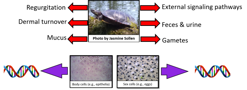
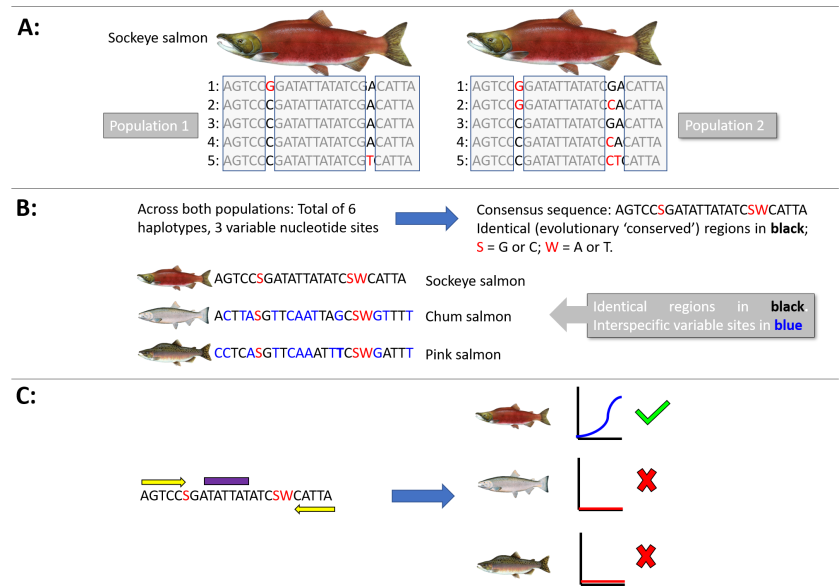
At least 5 individuals from each population (an isolated watershed or river, for example) should be characterized at the genetic marker level for diagnostic DNA differences (see Figure). The aim is to capture most of the naturally occurring genetic variation from which we can identify regions of the marker sequence that will amplify, via qPCR, all individual haplotypes from this species. This includes precluding any sequences which exhibit the signs of being what is called a ‘pseudogene’ – which is a mitochondrial marker that has, in the evolutionary distant past, been inserted into the nuclear genome and evolves independently from its functional analog[5]. To do so, a consensus sequence can be constructed that incorporates all the identical portions of the genetic marker shared across haplotypes to be identified as potential binding sites for short DNA sequences (primers and probes) that act as target species-specific identifiers for qPCR detection.

Now that we have isolated sequences that can be used to detect all of the within-species genetic marker variants, the next stage is to ensure there is enough genetic divergence at these target-specific binding sites to preclude the erroneous amplification of non-target species – i.e., there should be a significant number of nucleotide differences between the target and the non-target species. Non-target species to be considered are often those that share a recent evolutionary history (e.g., species within the same genus or sub-family, and those that share similar habitat preferences). In our hypothetical example, we collate all the same marker sequences for all co-distributed salmonid fishes, and perhaps other more distant relatives (e.g., smelts and pikes) that display overlap in ecological niches and habitat preferences (In the Figure, we show just two consensus non-target species sequences belonging to two congeneric Oncorhynchus species (chum and pink salmon) for ease of illustration). Moreover, we also need to consider these co-distributed species assemblages for every single waterbody in which the target is found, so that the assay will work in all known locations. This requires significant investment in generating sequence data of eDNA marker sequences for a wide array of species across a range of aquatic habitats.

Figure: A schematic diagram showing how homologous sequence variation within and among species may be used to design a generic species-specific qPCR assay to amplify the sockeye salmon (Oncorhynchus nerka) for eDNA surveys of two populations. A: The genetic marker of choice is sequenced for five individuals from each of the two populations. All haplotypes and variable nucleotide sites are identified. In this hypothetical example, the short 24 base pair fragment of the maker gene yields 3 haplotypes in population 1 based on two variable sites, and 5 haplotypes from population 2 based on 3 variable sites. The variable sites are identified by red typeface in the collated sequences, whereas the identical, or evolutionary conserved, sites are boxed in grey. Population 2 has a site-specific substitution that is diagnostic of that population, and 2 haplotypes are common to both populations. B: From these ten sequences, 6 haplotypes have been identified across 3 variable sites. The consensus sequence identifies the conserved regions which can be used to design the primers and probes. In this example, the sequence is too short for a real assay to be designed, but the concept can be perfectly illustrated. The “S’ and “W” represent codes for what type of nucleotide (e.g., W = A or T) is present at that site across all individuals within the species, if it is not shared amongst all haplotypes. We can then align this consensus sequence with that of co-distributed species (here, chum and pink salmon) to identify if there are enough base pair differences in the sockeye conserved regions with those of the non-target species. These sites are shown in blue. In a subsequent post, we will discuss in more detail how many differences are optimal for assay specificity, but in this example > 30-40% of nucleotide sites are divergent in the primer (C: yellow bars) and probe (purple bar) sites, so that the assay should only result in a qPCR amplification curve of the sockeye salmon. If there are not enough divergent sites between the sockeye salmon and the chum and pink salmon regions to result in species-specific amplification, then another marker gene must be analyzed for suitability. The more genomic information available for analysis, the more robust the assay that can be designed.

Even distantly related species should be considered because of the phenomenon of ‘saturation’ – a term that addresses the fact that at every single nucleotide site that is shared between species, there are only four possible states – that is to say, one of the four nucleotide bases: A, C, G or T.  During the course of evolution, these loci may mutate and can change into one of the three other bases, so on and so forth down the ages. However, the probability that an original ‘A’ base will mutate back to that state later in its evolutionary history, and to be recorded in that state in contemporary populations, becomes non-trivial as the generations pass, and is especially true of sites that have elevated rates of nucleotide substitution (e.g., including some of the genes used as eDNA markers)[6]. In some instances, high rates of nucleotide saturation lead to what is known as ‘long-branch attraction’, whereby even distantly related species (i.e., those on distant (long) ‘branches’ of species’ family trees (called a ‘phylogeny’)) are inferred to be more closely related than they actually are (the ‘branches’ are artefactually drawn closer together in the reconstructed phylogeny)[7].

In population genetic studies, there are ways to incorporate nucleotide site saturation into evolutionary models of sequence variation, but for designing molecular biology markers, we have to incorporate this phenomenon into our database curation to ensure non-amplification of distantly taxa, including choosing a suitable marker for the taxon of interest. For instance, for recently derived taxa, it is ok to choose a highly evolving segment of the mitochondrial genome (e.g., the D-loop within the frog genus Pseudacris, for example), however, it might be inappropriate to use the D-loop for genera or sub-families with relatively deep evolutionary histories (e.g., salmonid fishes, whose origins extend tens of millions of years into the past[8]).

Coda

In this post, we have broadly discussed gathering and curating data for designing a species-specific assay to be generally deployed across a species’ range, or at least in the populations from which sequence data were generated. Here at PBI, we are also developing novel ways to tease apart even extremely closely-related species with low levels of nucleotide variation. In a similar vein, we also hope to design population-specific assays that may be able to target individual evolutionary significant units (ESUs) and management or conservation units (M/CUs)[9].

In the next blog, we shall develop further the required minimal standards of a reliable, robust and reputable eDNA qPCR assay, and how these requirements extend and embellish those of the MIQE guidelines. We shall treat in some detail the concepts LOD (limit of detection) and LOQ (limit of quantification) and ask: what are the crucial assay requisite parameters (CARP) for designing, optimizing and validating eDNA assays?

[1] Bustin et al. (2009). The MIQE guidelines: minimum information for publication of qPCR experiments. Clinical Chemistry 55, doi.org/41373/clinch.2008.112797.

[2] Lahoz-Monfort et al. (2015). Statistical approaches to account for false positive errors in environmental DNA samples. Molecular Ecology Resources, 16, doi: 10.1111/1755-0998.12486.

[3] Hale et al. (2012). Sampling for Microsatellite-Based Population Genetic Studies: 25 to 30 individuals per population Is enough to accurately estimate allele frequencies.  PloS One, doi: 10.1371/journal.pone/0045170

[4] Luo et al. (2018). Biparental inheritance of Mitochondrial DNA in humans. Proceedings of the National Academy of Sciences, doi: 10.1073/pnas.1810946115

[5] Benasson et al. (2001). Mitochondrial pseudogenes: evolution’s misplaced witnesses. Trends in Ecology and Evolution, 16, 314-321.

[6] Smith & Smith (1996). Synonymous nucleotide divergence: what is “saturation”? Genetics, 142, 1033-1036.

[7] Felsenstein J (2003). Inferring Phylogenies, Sunderland (Sinauer).

[8] Crête-Lafrenière et al. (2012). Framing the Salmonidae family phylogenetic portrait: a more complete pictire from increased taxon sampling. PloS One, doi: 10.1371/journalpone.0046662.

[9] Palsbøll et al. (2006). Identification of management units using population genetic data. Trends in Ecology and Evolution, 22, 11-16.

Using Environmental DNA (eDNA) to Monitor Aquatic Ecosystems

Environmental DNA monitoring – eDNA – is at the vanguard of a new wave of technologically advanced monitoring efforts. With roots in soil and paleoecology, eDNA was first used to detect a multicellular aquatic organism– the invasive American bullfrog Lithobates catesbeianus– in a landmark scientific paper by Ficetola et al. in 2008[1]. By applying the widely used, yet highly sensitive, polymerase chain reaction (PCR) – a reaction that ‘amplifies’ a specific DNA sequence in a sample, only if the species’ DNA is present in however little amount – Ficetola and colleagues detected the frogs’ DNA in sediment filtered out of the water column. To understand why, a current working definition of eDNA – adopted by most ecologists – will illuminate: eDNA is “…genetic material obtained directly from environmental samples (soil, sediment, water, etc.) without any obvious signs of biological source material” (Thomsen & Willerslev 2015[2]). Examples of how eDNA is shed by an organism – e.g., here a midland painted turtle Chrysemys picta – are illustrated in the figure below.

In the figure, DNA-containing cells are constantly or periodically shed from the internal linings of the turtle’s gut, reproductive system, through regurgitation of food, the replacement of skin cells and mucus, the egress of waste materials, and through the release of sex cells (i.e., sperm and eggs). Once in the water, DNA is somewhat protected within cells. Eventually, cells are broken down and DNA is released into the aqueous environment whereupon it is to be found in solution. Although eDNA is depleted through a number of biological, chemical and physical processes, it will keep being replenished if the organism is still to be found living in the vicinity. That is to say, the signal of eDNA will be stronger the closer it is to its source, and will also increase when there are more individuals in a local population, if the volume of water remains the same. Therefore, an eDNA signal can be a reliable indicator of the target species’ presence in a given habitat.

What are the chief benefits of eDNA monitoring? First of all, there is no need to physically sample the species, thus minimising disturbance associated by the targeted monitoring of live creatures that are sensitive to stress. Furthermore, as only water samples are taken, and by few people, there will be a decrease in the environmental footprint associated with monitoring efforts per se. Because PCR is a highly sensitive molecular biological assay, eDNA surveys tend to have much higher sensitivities to be able to detect rare or cryptic species than conventional methods (e.g., Schmelzle & Kinziger 2016[3]). As a result, species-specific eDNA surveys are also potentially much more cost-effective than conventional techniques. Furthermore, anyone can take a water sample, following simple instructions, democratising and facilitating citizen science projects across the globe. Indeed, the current crop of companies that offer eDNA detection services are predicated on a model of water samples being collected by lay and technical personnel for processing back in a central laboratory.

However, as eDNA is a nascent technology, uncertainty exists over some of the conclusions drawn from early eDNA studies. However, these issues (i.e., sources of ‘error’) are under ongoing scrutiny by scientists, including here at Precision Biomonitoring, to minimise their impacts. As such, all potential sources of error, as they are currently understood, must be acknowledged and incorporated into any technical development (i.e., design, production and validation of species-specific PCR assays) or standard operating protocols for field surveys. For example, organisms are liable to move throughout their lifetimes. Seasonality has shown to be a strong factor in eDNA detection success (de Souza et al. 2016[4]). It is imperative that surveys are conducted with a thorough knowledge of a species’ ecology, including insight into current distributions and habitat preferences, otherwise inadequate surveying will lead to a false negative result, i.e., inferring a target to be absent when it actually is present; just undetected. Failure to account for false negatives can result in severe financial repercussions if infrastructure projects are subsequently halted, put on-hold or abandoned due to the rediscovery of the target by an intrepid ecologist or member of the public. False negatives can also result from improper assay development, the underestimation of within-species genetic diversity at PCR amplification sites, and by the current disjointed process by which eDNA samples are processed by the majority of eDNA practitioners.

As noted previously, eDNA will decay if left exposed to natural world processes. Therefore, collected eDNA is at risk of post-sampling decay, as there would be no mechanism for eDNA replenishment in the collection vessel, reducing the eDNA signal and potentially failing to garner a positive PCR result. Therefore the risk of eDNA degradation during sampling – particularly on hot, sunny days – and in transit from the field to the laboratory, is highly significant. Inappropriate storage may also destroy eDNA (e.g., water crystal formation during freezing may ‘shred’ DNA molecules). To compound the status quo further, despite the best efforts of contemporaneous laboratories, there remains a significant risk of false positive PCR results mediated by the transportation of aerosolised DNA particles among labs within buildings through ventilation pathways. Most eDNA practitioners seek to physically separate the processing of eDNA samples (e.g., filter papers or precipitated water samples) with downstream PCR detection, but even that is far from fool-poof.

Here at Precision Biomonitoring, we are set to unveil a state-of-the-art platform that will seek to eliminate, or minimise, these sources of eDNA analytical and sampling error, through the eradication of transit stages to a central laboratory and the application of standard operating procedures. Moreover, we will further the cause of a democratised biomonitoring field in which no technical specialty is required to conduct sophisticated PCR-based species-specific assays. Our system, using bespoke PCR assays, will yield PCR eDNA results in real-time (< 2 hours from water sampling to PCR read-out), which can then be immediately disseminated to colleagues via the cloud.

It is our aim to give those working at the coalface of biodiversity monitoring (from professional ecologists to local citizen science projects), the power to conduct highly rigorous, and potentially highly coordinated, targeted eDNA surveys to better vouchsafe our world’s biodiversity heritage for all generations to come.

[1] Ficetola et al. (2008). Species detection using environmental DNA from water samples. Biology Letters, 4, 423-425.

[2] Thomsen & Willerslev (2015). Environmental DNA – An emerging tool in conservation for monitoring past and present biodiversity. Biological Conservation, 183, 4-18.

[3] Schmelzle & Kinziger (2016). Using occupancy modelling to compare environmental DNA to traditional field methods for regional-scale monitoring of an endangered aquatic species. Molecular Ecology Resources, 16, 895-908.

[4] de Souza et al. (2016). Environmental DNA (eDNA) detection probability is influenced by seasonal activity of organisms. PLoS One, doi: 10.1371/journal.pone.0165273